How to Compare 2 Columns in Excel​: Quick and Easy Guide

To compare two columns in Excel, use the formula =A1=B1 in a new column. This returns TRUE or FALSE based on the comparison.

Comparing columns in Excel is essential for data analysis. Whether you’re matching lists, verifying entries, or identifying discrepancies, this task is common in various fields. Excel offers efficient methods to compare columns, saving time and reducing errors. Understanding how to compare columns can streamline your workflow, making data management more effective.

This guide will walk you through the process, ensuring you can quickly and accurately compare columns in Excel. By mastering these techniques, you’ll enhance your data handling skills and improve overall productivity.

Credit: www.educba.com

Preparing Your Data

Before comparing two columns in Excel, prepare your data properly. This ensures accurate results and an easy comparison process.

Cleaning Your Data

Clean data is crucial for accurate comparisons. Follow these steps:

• Remove any empty rows and columns.
• Ensure there are no extra spaces in cells.
• Check for and remove any duplicate entries.
• Make sure all data is in the same format.

Use Excel’s built-in Trim function to remove extra spaces:

=TRIM(A1)

Replace A1 with the actual cell reference.

Setting Up Columns

Set up your columns correctly for easy comparison:

1. Ensure both columns are side by side.
2. Label each column for clarity.
3. Check that the data types match.
4. Align data in both columns.

Here is an example table:

Column A	Column B
Apple	Apple
Banana	Orange
Cherry	Cherry

With clean and well-set columns, you can start the comparison process.

Credit: www.shiksha.com

Using Conditional Formatting

Using Conditional Formatting in Excel is a powerful way to compare two columns. It helps you easily spot differences and similarities. This method is efficient and visually appealing.

Highlighting Differences

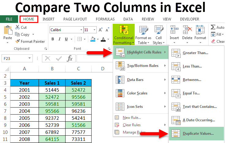
To start, select the range of cells you want to compare. Go to the Home tab and click on Conditional Formatting. Choose New Rule from the dropdown menu.

In the New Formatting Rule dialog box, select Use a formula to determine which cells to format. Enter the formula to compare the two columns. For example:

=A1<>B1

This formula checks if the cells in Column A are not equal to the cells in Column B. Click on the Format button, choose a fill color, and click OK. This will highlight the differences between the two columns.

Customizing Highlight Rules

To make your comparison more specific, you can customize the highlight rules. After selecting New Rule, use different formulas. For example, to highlight cells where Column A is greater than Column B:

=A1>B1

Choose a different fill color to distinguish this condition. You can also use multiple rules to highlight different conditions. This makes your data analysis more detailed and insightful.

Conditional Formatting in Excel can be customized further using icons, data bars, and color scales. These features allow more visual representation of your data. For instance, you can use a green fill for positive differences and red for negative ones.

Condition	Formula	Format
Highlight Differences	=A1<>B1	Yellow Fill
Column A > Column B	=A1>B1	Green Fill
Column A < Column B	=A1	Red Fill

With these steps, comparing columns in Excel becomes straightforward. Conditional Formatting provides a visual way to understand your data. This makes Excel a powerful tool for data analysis.

Using Formulas

Comparing two columns in Excel can be done easily using formulas. This method is efficient and saves a lot of time. Here, we will explore two main formulas: IF Function and VLOOKUP Function. These formulas help in identifying matches and differences between columns.

If Function

The IF Function is straightforward for comparing two columns. It checks if the values are equal and returns a specified result.

Here’s how to use it:

1. Select the cell where you want the result.
2. Enter the formula: =IF(A2=B2, "Match", "No Match")
3. Press Enter and drag the fill handle to apply the formula to other cells.

This formula compares the values in cells A2 and B2. If they match, it shows “Match”. If not, it shows “No Match”.

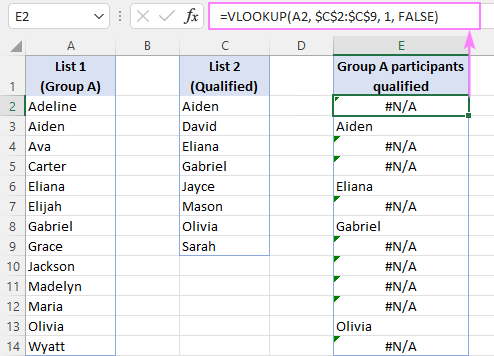
Vlookup Function

The VLOOKUP Function is more advanced. It searches for a value in a column and returns a corresponding value from another column.

Follow these steps:

1. Click on the cell where you want the result.
2. Enter the formula: =VLOOKUP(A2, B:B, 1, FALSE)
3. Press Enter and drag the fill handle to apply the formula to other cells.

This formula looks for the value in cell A2 within column B. If it finds a match, it returns the value. Otherwise, it returns an error.

Using these formulas, you can easily compare two columns in Excel. This helps in data analysis and validation tasks.

Using Excel’s Built-in Tools

Comparing two columns in Excel can be easy with built-in tools. These tools help you find differences and similarities quickly. You can use them to save time and effort.

Go To Special

The Go To Special feature helps you find cells with specific characteristics. To use this tool, follow these steps:

1. Select the first column you want to compare.
2. Press Ctrl + G to open the Go To dialog box.
3. Click on the Special button.
4. Select Row differences and click OK.

Excel will highlight the cells that are different between the two columns.

Remove Duplicates

The Remove Duplicates feature helps you find unique values. To use this tool, follow these steps:

1. Select the columns you want to compare.
2. Go to the Data tab on the Ribbon.
3. Click on the Remove Duplicates button.
4. In the dialog box, check the columns you want to compare.
5. Click OK.

Excel will show a message with the number of duplicate values removed.

Tool	Purpose
Go To Special	Highlight different cells between columns
Remove Duplicates	Find unique values in columns

Comparing Large Data Sets

Comparing large data sets in Excel can be challenging. This guide will help you understand how to compare two columns efficiently. With the right tools, you can manage even the largest data sets with ease.

Pivot Tables

Pivot Tables are powerful for comparing large data sets. They help summarize and analyze the data quickly.

To create a Pivot Table:

1. Select your data range.
2. Go to the Insert tab.
3. Click on PivotTable.
4. Choose where you want the Pivot Table to be placed.
5. Click OK.

Now, you can drag and drop fields to compare data.

Excel Add-ins

Excel Add-ins can extend the functionality of Excel. They are great for comparing large data sets.

Some popular Add-ins include:

• Power Query: Helps combine and transform data.
• Fuzzy Lookup: Compares and matches similar text strings.

To install an Add-in:

1. Go to the File tab.
2. Click on Options.
3. Select Add-ins.
4. Click Go next to Manage Excel Add-ins.
5. Check the box next to your desired Add-in.
6. Click OK.

With these tools, comparing data becomes much easier.

Credit: www.ablebits.com

Automating The Process

Automating the process of comparing two columns in Excel can save time and reduce errors. Instead of manually comparing data, you can use automated tools. These tools help you find differences and similarities quickly. Let’s explore some methods to automate this task.

Macros

Macros are powerful tools in Excel. They allow you to automate repetitive tasks. You can create a macro to compare two columns. Follow these steps to create a macro:

1. Open Excel and press Alt + F11 to open the Visual Basic for Applications (VBA) editor.
2. Click on Insert then Module.
3. Copy and paste the following code:

Sub CompareColumns()
    Dim i As Integer
    For i = 1 To 10 ' Adjust range as needed
        If Cells(i, 1).Value = Cells(i, 2).Value Then
            Cells(i, 3).Value = "Match"
        Else
            Cells(i, 3).Value = "No Match"
        End If
    Next i
End Sub

4. Press F5 to run the macro.

Third-party Tools

Third-party tools offer advanced features for comparing columns. These tools can handle large datasets and provide detailed reports. Below are some popular third-party tools:

• Power Query: An Excel add-in that simplifies data comparison.
• XL Comparator: A web-based tool for comparing Excel files.
• Spreadsheet Compare: Part of the Microsoft Office suite.

Using these tools can enhance efficiency. They also provide more options and flexibility for data analysis.

Troubleshooting

Comparing two columns in Excel can sometimes lead to problems. Understanding common errors and tips for accuracy can help. This section will guide you through troubleshooting these issues.

Common Errors

When comparing two columns, you might encounter some common errors. These errors can disrupt your workflow. Here are a few to watch out for:

• #N/A: This error means a value is not available. Check if the value exists in both columns.
• #VALUE!: This error occurs when the data types do not match. Ensure both columns have the same data type.
• Spaces: Extra spaces can cause mismatches. Trim the data to remove extra spaces.

Tips For Accuracy

Accuracy is crucial when comparing columns. Here are some tips to ensure precise comparisons:

1. Use Exact Function: This function checks if two values are exactly the same. It is case-sensitive and ensures accuracy.
2. Conditional Formatting: Highlight duplicates or unique values with conditional formatting. This helps visualize differences quickly.
3. Sort Data: Sort both columns in ascending or descending order. This makes it easier to spot differences.
4. Remove Duplicates: Use the ‘Remove Duplicates’ feature to clean your data. This ensures only unique entries remain.

Following these steps can help avoid common errors and improve accuracy. Troubleshooting becomes easier with these tips.

Frequently Asked Questions

How Do I Compare Two Columns In Excel?

To compare two columns in Excel, you can use the IF function. Enter the formula `=IF(A1=B1, “Match”, “No Match”)` in a new column. This will show if the cells in each row match.

Can Excel Highlight Differences Between Columns?

Yes, Excel can highlight differences between columns. Use Conditional Formatting with a formula like `=$A1$B1` to highlight cells that don’t match. This makes it easy to see discrepancies.

Is There A Quick Way To Find Duplicates?

Yes, you can quickly find duplicates using Conditional Formatting. Select the columns, go to “Home” > “Conditional Formatting” > “Highlight Cells Rules” > “Duplicate Values”. This will highlight all duplicate entries.

Can I Compare Columns Using Vlookup?

Yes, VLOOKUP can compare columns. Use `=VLOOKUP(A1, B:B, 1, FALSE)` to check if a value in column A exists in column B. This function helps in finding matches between columns.

Conclusion

Mastering how to compare two columns in Excel boosts productivity. Follow the steps to streamline your data analysis. Practice these techniques to enhance your Excel skills. By using these methods, you can save time and minimize errors. Keep exploring Excel’s features for efficient data management.

Happy comparing!