
To calculate the end of the year in Excel, use the formula =DATE(YEAR(TODAY()), 12, 31). This formula returns December 31 of the current year.
Excel provides powerful tools for date calculations, including the ability to determine the end of the year. The end-of-year formula, =DATE(YEAR(TODAY()), 12, 31), simplifies this task by automatically generating December 31 for the current year. This function is useful for financial reporting, project timelines, and planning activities that require precise year-end dates.
By mastering this formula, users can enhance their Excel skills and improve efficiency in managing time-sensitive data. Excel’s versatility makes it an invaluable resource for both personal and professional use.
Credit: www.educba.com
Introduction To Year-end Calculations
Year-end calculations are crucial for businesses. They help in closing the financial year. Using Excel for these tasks can save time. Excel’s formulas and functions make the process easier. Let’s dive into the importance of year-end calculations.
Importance Of Year-end Calculations
Year-end calculations ensure your financial data is accurate. They help identify profits and losses. This process is essential for preparing financial statements. Accurate calculations aid in tax filing. They also help in planning for the next year.
- Ensures data accuracy
- Identifies profits and losses
- Prepares financial statements
- Aids in tax filing
- Helps in future planning
Common Year-end Tasks
Year-end tasks often involve several steps. These steps ensure your accounts are in order. Here are some common tasks:
- Reconcile bank statements
- Review accounts receivable and payable
- Update inventory records
- Calculate depreciation
- Prepare financial statements
Using Excel can simplify these tasks. Excel’s formulas can automate calculations. Here’s a table showing some useful formulas:
| Task | Excel Formula |
|---|---|
| Sum of values | =SUM(range) |
| Average of values | =AVERAGE(range) |
| Depreciation calculation | =SLN(cost, salvage, life) |
| Net profit margin | = (NetIncome / Revenue) 100 |
These formulas can save time and reduce errors. They make year-end calculations more efficient. Start using Excel for your year-end tasks today.
Credit: www.ablebits.com
Basic Excel Formulas For Year-end
The end of the year is a busy time for many. Managing data in Excel can be easier with the right formulas. Basic Excel formulas help summarize and analyze data quickly.
Sum And Sumif
Use the SUM formula to add up numbers in a range. It’s simple and efficient.
=SUM(A1:A10)
The SUMIF formula adds numbers based on a condition. This is useful for specific data.
=SUMIF(A1:A10, ">=10")
With these formulas, you can manage your year-end data easily.
Average And Averageif
The AVERAGE formula calculates the mean of numbers in a range. It’s very useful for finding the average value.
=AVERAGE(B1:B10)
The AVERAGEIF formula calculates the mean based on a condition. This helps to find the average of specific data.
=AVERAGEIF(B1:B10, ">=10")
Using these formulas, you can quickly analyze your year-end data.
Advanced Excel Formulas
Mastering advanced Excel formulas can make your data analysis faster and easier. These formulas help you handle complex tasks with ease. Let’s explore some powerful formulas!
Vlookup And Hlookup
VLOOKUP stands for Vertical Lookup. It searches for a value in the first column and returns a value in the same row from a specified column.
=VLOOKUP(lookup_value, table_array, col_index_num, [range_lookup])For example, =VLOOKUP(A2, B2:D10, 3, FALSE) searches for the value in A2 and returns the value from the third column.
HLOOKUP stands for Horizontal Lookup. It searches for a value in the first row and returns a value in the same column from a specified row.
=HLOOKUP(lookup_value, table_array, row_index_num, [range_lookup])For example, =HLOOKUP(A1, B1:F5, 4, TRUE) searches for the value in A1 and returns the value from the fourth row.
Index And Match
The INDEX and MATCH functions together are powerful alternatives to VLOOKUP and HLOOKUP.
INDEX returns the value of a cell in a specified table based on the row and column numbers.
=INDEX(array, row_num, [column_num])For example, =INDEX(A1:D10, 2, 3) returns the value from the second row and third column.
MATCH searches for a specified value in a range and returns its relative position.
=MATCH(lookup_value, lookup_array, [match_type])For example, =MATCH("apple", A1:A10, 0) returns the position of “apple” in the range A1:A10.
Combining INDEX and MATCH allows for more flexible and dynamic lookups.
=INDEX(return_range, MATCH(lookup_value, lookup_range, 0))For example, =INDEX(B1:B10, MATCH("apple", A1:A10, 0)) returns the corresponding value in column B where “apple” is found in column A.
Automating Year-end Calculations
Year-end calculations can be challenging. Excel can help automate these tasks. This reduces errors and saves time. Excel has powerful tools like macros and VBA scripts.
Using Macros
Macros record your actions in Excel. You can replay these actions later. This is great for repetitive tasks. Follow these steps to create a macro:
- Go to the Developer tab.
- Click on Record Macro.
- Perform the actions you want to automate.
- Click on Stop Recording.
Now, you can run this macro anytime. It will repeat your recorded actions.
Implementing Vba Scripts
VBA scripts give you more control than macros. You can write custom code to automate tasks. Here is a simple VBA script example:
Sub YearEndSummary()
    Dim ws As Worksheet
    Set ws = ThisWorkbook.Sheets("Sheet1")
    ws.Cells(1, 1).Value = "Year-End Summary"
    ws.Cells(2, 1).Value = "Total Sales"
    ws.Cells(2, 2).Formula = "=SUM(B2:B12)"
End Sub
To use this script:
- Open the VBA editor (Alt + F11).
- Insert a new module.
- Copy and paste the script.
- Run the script.
This script creates a year-end summary. It calculates total sales and displays it.
Data Visualization Techniques
Visualizing data in Excel helps make sense of complex information. Using the right techniques, you can highlight trends and insights effectively. This section covers two essential techniques: Creating Charts and Using PivotTables.
Creating Charts
Charts are a powerful tool for visualizing data. They make it easy to understand and compare data.
- Bar Charts: Great for comparing different groups.
- Line Charts: Perfect for showing trends over time.
- Pie Charts: Useful for displaying parts of a whole.
To create a chart in Excel:
- Select your data range.
- Go to the Insert tab.
- Choose the chart type you need.
Excel will generate the chart automatically. You can then customize it as needed.
Using Pivottables
PivotTables summarize large datasets quickly. They help in data analysis and finding patterns.
Steps to create a PivotTable:
- Select your data range.
- Go to the Insert tab.
- Click on PivotTable.
- Choose where to place the PivotTable.
- Drag fields to the Rows and Columns areas.
PivotTables can perform calculations like sums, averages, and counts.
Using both charts and PivotTables can provide a comprehensive view of your data.
Error Checking And Troubleshooting
Working with Excel formulas can sometimes lead to unexpected errors. Troubleshooting and correcting these errors is crucial. This section will guide you through Error Checking and Troubleshooting in Excel, focusing on common formula errors and debugging techniques.
Common Formula Errors
Excel formulas can produce various errors. Below is a table of common errors and their meanings:
| Error | Meaning |
|---|---|
| #DIV/0! | Division by zero. |
| #VALUE! | Wrong type of argument. |
| #REF! | Invalid cell reference. |
| #NAME? | Unrecognized text in the formula. |
| #N/A | Value is not available. |
Debugging Techniques
Below are some effective techniques for debugging Excel formulas:
- Use the Evaluate Formula tool to step through the formula.
- Check for extra spaces or typos in your formula.
- Verify that all cell references are correct and not broken.
- Use the IFERROR function to catch and manage errors.
- Break down complex formulas into simpler parts to isolate issues.
By understanding these common errors and using these debugging techniques, you can resolve most issues. This ensures your Excel formulas work correctly and efficiently.
Best Practices For Year-end Reporting
Year-end reporting can be a daunting task. Following best practices ensures smooth and accurate reporting. These practices help in organizing and verifying data efficiently.
Organizing Data
Proper data organization is crucial for year-end reports. Start by creating a structured Excel sheet. Use clear headings and consistent formats for easy navigation.
Here are some tips for organizing data:
- Use descriptive column names.
- Maintain a consistent date format.
- Group similar data together.
- Use filters and sorting options for quick access.
Organizing data in Excel helps in quick analysis. It also reduces errors during reporting.
Ensuring Data Accuracy
Ensuring data accuracy is vital. Incorrect data can lead to wrong decisions. Here are some steps to ensure data accuracy:
- Regularly update your data.
- Use formulas to automate calculations.
- Perform data validation checks.
- Double-check entries for typos and errors.
Using Excel formulas like SUMIF, COUNTIF, and VLOOKUP can help verify data. These formulas ensure all data is accounted for.
Here is a simple example:
| Formula | Purpose |
|---|---|
=SUMIF(range, criteria, sum_range) | Adds values based on criteria |
=COUNTIF(range, criteria) | Counts cells based on criteria |
=VLOOKUP(lookup_value, table_array, col_index_num, [range_lookup]) | Finds data in a table |
Remember to regularly backup your data. This prevents loss and ensures safety.
Following these best practices makes year-end reporting efficient. Organize and verify your data for accurate results.

Credit: community.smartsheet.com
Case Studies And Examples
The End of Year Formula in Excel is a powerful tool. Many users utilize it to streamline their financial processes. This section delves into real-world applications and success stories. It showcases how individuals and companies use this formula effectively.
Real-world Applications
Many businesses use the End of Year Formula for various purposes. Here are a few examples:
- Financial Reporting: Companies summarize their annual financial data.
- Budgeting: Organizations set budgets for the upcoming year.
- Performance Analysis: Managers review employee performance over the year.
Consider a small business tracking its sales. They use the formula to calculate total sales for the year. This helps them identify trends and plan for the future. Another example is a school using it for student performance reports. They aggregate scores to identify top performers.
Success Stories
Many have achieved significant success using the End of Year Formula. Let’s explore a few inspiring stories:
- Case Study 1:
- Case Study 2:
- Case Study 3:
XYZ Corp used the formula to track annual expenses. They reduced costs by 15% the next year.
ABC Nonprofit tracked donations and funds. They increased annual donations by 20% using insights from the formula.
LMN School improved student performance tracking. They identified key areas for improvement and boosted grades by 10%.
These stories highlight the formula’s practical impact. By leveraging the End of Year Formula, organizations can achieve significant improvements.
Frequently Asked Questions
How To Create An End Of Year Formula In Excel?
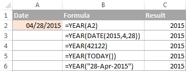
Use the DATE function with the YEAR, MONTH, and DAY functions to calculate end of year dates.
What Is The End Of Year Date Formula?
Use the formula `=DATE(YEAR(A1),12,31)` to get the end of year date.
Can Excel Calculate Fiscal Year End?
Yes, use a custom formula to calculate the fiscal year end based on your fiscal calendar.
How To Handle Leap Years In Excel?
Excel’s DATE function automatically adjusts for leap years when calculating end of year dates.
How To Use Eomonth Function For Year-end?
EOMONTH can help find the last day of any month, use `=EOMONTH(A1, 11)` for December.
What Are Common Errors In Year-end Formulas?
Common errors include incorrect cell references and not accounting for leap years. Double-check your formulas.
Conclusion
Mastering the end of year formula in Excel can enhance productivity. It’s a valuable tool for data analysis. Implementing this formula helps streamline annual reports and financial summaries. Practice regularly to gain confidence and improve efficiency. Start using it today to simplify your year-end tasks and boost your Excel skills.