
ANOVA in Excel helps compare means across multiple groups to determine if they are statistically different. It is a valuable tool for data analysis.
ANOVA (Analysis of Variance) is a statistical method used to analyze differences among group means in a sample. Excel offers built-in features to perform ANOVA, making it accessible and straightforward. You can find the ANOVA tools within the Data Analysis Toolpak.
This tool is essential for researchers and analysts who need to understand variations within their data. It supports various applications, from scientific research to business analytics. Using ANOVA in Excel, you can efficiently handle large datasets and derive meaningful insights. This helps in making informed decisions based on statistical evidence.
Introduction To Anova
ANOVA, or Analysis of Variance, is a powerful statistical tool. It helps to determine if there are significant differences between the means of three or more groups. ANOVA in Excel simplifies this process, making data analysis accessible. Understanding ANOVA is key for anyone working with data.
What Is Anova?
ANOVA stands for Analysis of Variance. It is used to compare means. This method checks if at least one group mean is different. ANOVA is especially useful in experiments and research.
Using ANOVA, we can test hypotheses about data. It helps to understand if differences are statistically significant. This means the differences are not by chance.
Importance Of Anova In Data Analysis
ANOVA is crucial in data analysis. It helps find patterns and differences. With ANOVA, we can make informed decisions based on data.
Here are a few reasons why ANOVA is important:
- Detects Differences: Identifies if group means are different.
- Reduces Error: Minimizes the risk of Type I errors.
- Simple to Use: Easy to perform using Excel.
- Versatile: Applicable in various fields like marketing and medicine.
To perform ANOVA in Excel, follow these steps:
- Open your data in Excel.
- Click on the Data tab.
- Select Data Analysis from the Tools group.
- Choose ANOVA: Single Factor.
- Input your data range and click OK.
ANOVA in Excel provides results quickly. It shows the F-value and p-value. These values help determine if the differences are significant.
Setting Up Excel For Anova
Analysis of Variance (ANOVA) helps compare means across groups. Excel’s Analysis ToolPak makes this process straightforward. Follow these steps to set up Excel for ANOVA.
Installing Analysis Toolpak
The Analysis ToolPak is an add-in for Excel. It provides data analysis tools.
- Open Excel.
- Click on the File tab.
- Go to Options.
- Select Add-ins from the left pane.
- In the Manage box, choose Excel Add-ins and click Go.
- Check the box for Analysis ToolPak and click OK.
The ToolPak is now installed. You can access it from the Data tab.
Navigating Excel Interface
To perform ANOVA, you need to know where to find the tools.
First, go to the Data tab on the ribbon. Look for the Data Analysis button. This button opens the Analysis ToolPak.
Click on Data Analysis. A window will pop up with various analysis tools. Select ANOVA: Single Factor or ANOVA: Two-Factor based on your needs.
Click OK to proceed to the next steps. You will be prompted to input your data range and other parameters.
After setting the parameters, click OK. Excel will generate the ANOVA output on a new worksheet.
With these simple steps, you can set up Excel for ANOVA quickly.
Types Of Anova
ANOVA, or Analysis of Variance, is a statistical method used to compare means among groups. In Excel, you can perform different types of ANOVA to understand your data better. This section will focus on the Types of ANOVA you can use in Excel.
One-way Anova
One-Way ANOVA helps you compare the means of three or more groups. It checks if at least one group mean is different. You need one independent variable with multiple levels.
For example, you might compare test scores of students from three different classes. Here, the class is the independent variable, and the test score is the dependent variable.
- Step 1: Organize your data in columns.
- Step 2: Go to the Data tab.
- Step 3: Select Data Analysis and choose ANOVA: Single Factor.
- Step 4: Enter your data range and click OK.
Excel will then provide an output table showing F-statistic and p-value. A low p-value (typically <0.05) means at least one group mean is different.
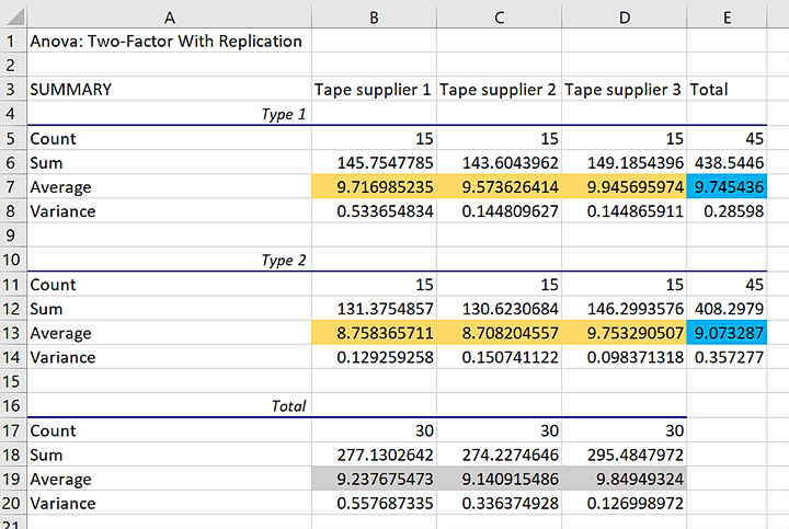
Two-way Anova
Two-Way ANOVA examines the effect of two independent variables on a dependent variable. It also checks for interaction between the two variables.
Imagine you want to study the effect of teaching method and study time on test scores. Here, teaching method and study time are the independent variables.
- Step 1: Arrange your data in a grid format.
- Step 2: Click on the Data tab.
- Step 3: Choose Data Analysis and select ANOVA: Two-Factor With Replication.
- Step 4: Enter your data range and replication info, then click OK.
Excel will generate an output table with F-statistics and p-values for each factor and their interaction. A low p-value for an interaction term suggests the two factors influence each other.
Both One-Way and Two-Way ANOVA are powerful tools in Excel for data analysis. They help you make sense of complex data sets easily.

Credit: mattchoward.com
Preparing Your Data
Before performing an ANOVA in Excel, you need to prepare your data. This involves organizing your data in a structured way and ensuring its accuracy. Proper preparation ensures reliable and meaningful results.
Organizing Data In Excel
First, you need to organize your data in a clear format. Create a new worksheet in Excel. Each column should represent a different group or category. Each row should represent a single observation or data point.
Here is an example of how to organize your data:
| Group 1 | Group 2 | Group 3 |
|---|---|---|
| 5 | 6 | 7 |
| 8 | 9 | 10 |
| 11 | 12 | 13 |
Ensuring Data Accuracy
Accurate data is crucial for reliable ANOVA results. Check your data for errors and inconsistencies. Ensure there are no blank cells within your data range.
Follow these steps to ensure data accuracy:
- Verify each data point for correctness.
- Remove any outliers or incorrect entries.
- Ensure all data points are numeric.
- Double-check for any blank cells.
By organizing and verifying your data, you set a strong foundation for performing ANOVA in Excel. Proper data preparation leads to accurate and meaningful analysis.
Performing One-way Anova In Excel
One-Way ANOVA in Excel helps compare means across multiple groups. It is useful to see if any group’s mean is different. Excel makes the process simple and quick.
Step-by-step Guide
Follow these steps to perform One-Way ANOVA in Excel:
- Open Excel and input your data in columns.
- Click on the Data tab in the ribbon.
- Select Data Analysis from the Analysis group.
- Choose Anova: Single Factor and click OK.
- In the dialog box, select your data range.
- Check the box for Labels in First Row if applicable.
- Select an output range or a new worksheet.
- Click OK to run the analysis.
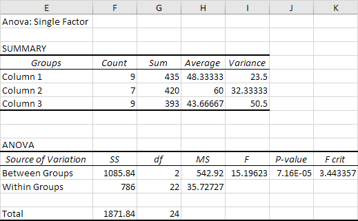
Interpreting Results
After running ANOVA, Excel provides a table with results:
| Source of Variation | SS | df | MS | F | P-value | F crit |
|---|---|---|---|---|---|---|
| Between Groups | SS Between | df Between | MS Between | F Value | P-value | F crit |
| Within Groups | SS Within | df Within | MS Within | |||
| Total | Total SS | Total df |
Focus on the P-value. If the P-value is less than 0.05, the means are different. The F Value and F crit help confirm this. Compare the F Value with F crit. If the F Value is greater, the means are different.
Performing Two-way Anova In Excel
Two-Way ANOVA is a powerful statistical tool. It helps to analyze the interaction between two independent variables. Performing Two-Way ANOVA in Excel is straightforward and efficient.
Step-by-step Guide
Follow these steps to perform Two-Way ANOVA in Excel:
- Open Excel and enter your data into a table.
- Click on the “Data” tab.
- Select “Data Analysis” from the Analysis group.
- Choose “ANOVA: Two-Factor with Replication” and click “OK”.
- Input the range of your data in the “Input Range” field.
- Set the “Rows per sample” according to your data.
- Select the output range where you want to see the results.
- Click “OK” to run the analysis.
Interpreting Results
After running the analysis, you will see a table with several key values:
| Source of Variation | SS | df | MS | F | P-value | F crit |
|---|---|---|---|---|---|---|
| Rows | Sum of squares for rows | Degrees of freedom for rows | Mean square for rows | F-value for rows | P-value for rows | Critical value for rows |
| Columns | Sum of squares for columns | Degrees of freedom for columns | Mean square for columns | F-value for columns | P-value for columns | Critical value for columns |
| Interaction | Sum of squares for interaction | Degrees of freedom for interaction | Mean square for interaction | F-value for interaction | P-value for interaction | Critical value for interaction |
P-value is crucial for interpreting results. If the P-value is less than 0.05, the result is significant. This means the variables interact.
Analyze the F-value and F crit. If F-value is greater than F crit, it indicates significance.
Use these values to understand the relationship between variables. This helps in making informed decisions.
Common Mistakes And Troubleshooting
Performing Anova in Excel can be tricky. Many users face common mistakes and need troubleshooting tips. This section helps you avoid errors and solve issues.
Avoiding Common Errors
Many people make mistakes with data entry and formula use. Here are some tips to avoid these errors:
- Check Data Entry: Ensure no empty cells in your data range.
- Correct Format: Data should be in numeric format, not text.
- Data Range: Select the correct range for analysis.
- Consistent Groups: Each group should have the same number of data points.
Troubleshooting Tips
Even with precautions, errors can occur. Use these tips to troubleshoot:
- Error Messages: Check for any error messages and read them carefully.
- Recalculate: Sometimes recalculating the data helps fix errors.
- Check Formulas: Ensure all formulas are entered correctly.
- Update Excel: Make sure your Excel software is up-to-date.
| Common Errors | Solutions |
|---|---|
| Data Range Error | Recheck the selected data range. |
| Empty Cells | Ensure no empty cells in the data. |
| Incorrect Format | Convert data to numeric format. |
| Formula Errors | Check and correct the formulas. |
Credit: www.goskills.com
Advanced Tips And Tricks
Mastering ANOVA in Excel can elevate your data analysis skills. Let’s explore some advanced tips and tricks to enhance your proficiency. These include using multiple variables and visualizing ANOVA results.
Using Multiple Variables
Excel allows you to perform ANOVA with multiple variables. This is known as two-way ANOVA. It helps in analyzing the interaction between variables. Here are the steps to use multiple variables:
- Click on Data tab.
- Select Data Analysis tool.
- Choose Anova: Two-Factor With Replication.
- Input your data range.
- Set the number of Rows per sample.
- Click OK to run the analysis.
Using multiple variables helps to understand complex data relationships. It also improves the accuracy of your analysis.
Visualizing Anova Results
Visualizing ANOVA results can make data interpretation easier. Excel provides various tools for this purpose:
- Bar Charts: Use these to compare group means.
- Box Plots: These show data distribution and outliers.
- Interaction Plots: Visualize interactions between variables.
To create a bar chart:
- Select the Insert tab.
- Choose Bar Chart.
- Select your data range.
- Click OK to generate the chart.
For a box plot, follow these steps:
- Click on the Insert tab.
- Choose Box and Whisker chart.
- Input your data range.
- Click OK to create the plot.
Using these visualization tools can make your ANOVA results clearer and more understandable.
Practical Applications
ANOVA, or Analysis of Variance, is a powerful statistical tool. Using ANOVA in Excel helps businesses and researchers. It provides insights from complex data. Below, explore how ANOVA can be applied practically.
Business Use Cases
Businesses often use ANOVA in Excel to analyze sales data. For example, a company may want to compare sales across different regions. This helps identify which regions perform best.
Another application is in product testing. Companies can test different versions of a product. ANOVA helps in understanding which version performs better.
Marketing campaigns also benefit from ANOVA. Businesses can compare the effectiveness of various marketing strategies. This ensures they invest in the most effective ones.
| Business Application | ANOVA Use |
|---|---|
| Sales Analysis | Comparing regional sales performance |
| Product Testing | Evaluating different product versions |
| Marketing Campaigns | Assessing strategy effectiveness |
Academic Research Examples
In academic research, ANOVA in Excel is indispensable. It helps in comparing different groups. This is crucial in experiments with multiple variables.
Education studies often use ANOVA. Researchers compare test scores among different teaching methods. This reveals which method is most effective.
Healthcare research also relies on ANOVA. For example, comparing the effectiveness of different treatments. This ensures patients receive the best care.
- Education Studies: Comparing teaching methods
- Healthcare Research: Evaluating treatment effectiveness
- Psychology Experiments: Analyzing behavioral data
Credit: www.excel-easy.com
Frequently Asked Questions
How Do I Perform Anova In Excel?
To perform Anova in Excel, navigate to the “Data” tab. Select “Data Analysis” and choose “ANOVA. ” Input your data range and click “OK. “
What Is Anova Used For In Excel?
Anova in Excel is used to compare means of different groups. It helps determine if there are any statistically significant differences.
Can I Use Anova In Excel For Multiple Groups?
Yes, you can use Anova in Excel for multiple groups. It allows comparing more than two groups simultaneously.
How Do I Interpret Anova Results In Excel?
Interpret Anova results by looking at the p-value. A p-value less than 0. 05 indicates significant differences among groups.
Conclusion
Mastering Anova in Excel can boost your data analysis skills. It’s a valuable tool for comparing multiple groups. By following the steps outlined, you can easily perform Anova tests. This enhances your ability to make informed decisions. Start using Anova in Excel today to streamline your statistical analysis.