
To apply conditional formatting based on another cell in Excel, use the “New Rule” option in Conditional Formatting. Select “Use a formula to determine which cells to format.”
Conditional formatting in Excel enhances data visualization by applying specific formatting to cells that meet certain criteria. This feature is particularly useful for highlighting important information, identifying trends, or comparing data sets. By using conditional formatting based on another cell, users can create dynamic and visually appealing spreadsheets.
This method allows for greater flexibility and precision, ensuring that only relevant data is highlighted. It saves time and improves efficiency, making data analysis more intuitive and effective. Understanding how to leverage this tool can significantly enhance your productivity in Excel.
Getting Started
Excel Conditional Formatting is a powerful tool. It helps you highlight cells based on certain conditions. This guide will show you how to get started.
Opening Excel
First, you need to open Excel. Double-click on the Excel icon on your desktop. You can also search for Excel in your start menu.
Navigating To Conditional Formatting
Once Excel is open, find the Home tab. Under this tab, look for the Styles group. In this group, you will see the Conditional Formatting option. Click on it to open the menu.
Steps to Navigate
- Open Excel.
- Go to the Home tab.
- Find the Styles group.
- Click on Conditional Formatting.
Conditional Formatting Menu
The Conditional Formatting menu provides several options. You can choose from Highlight Cells Rules, Top/Bottom Rules, and more.
Choosing a Rule Type
- Highlight Cells Rules: Use this to highlight cells based on specific criteria.
- Top/Bottom Rules: Use this to highlight top or bottom values.
By following these steps, you can easily navigate to Conditional Formatting. This is the first step to applying formatting based on another cell.
Basic Rules
Excel’s Conditional Formatting is a powerful tool. It helps highlight important data based on specific criteria. Understanding the basic rules is essential for effective data analysis. This section covers how to format cells based on another cell’s value.
Highlight Cells Rules
The Highlight Cells Rules feature allows you to format cells that meet certain criteria. You can highlight cells based on their value, text, dates, and more.
- Greater Than: Highlight cells with values greater than a specified number.
- Less Than: Highlight cells with values less than a specified number.
- Between: Highlight cells with values between two numbers.
- Equal To: Highlight cells that match a specific number or text.
These rules are helpful for quickly identifying outliers or important data points. To apply, select the cells, go to the Home tab, click Conditional Formatting, and choose Highlight Cells Rules.
Top/bottom Rules
The Top/Bottom Rules feature highlights the highest or lowest values in a range. This is useful for identifying top performers or areas needing attention.
- Top 10 Items: Highlight the top 10 values in a range.
- Top 10%: Highlight the top 10% of values in a range.
- Bottom 10 Items: Highlight the bottom 10 values in a range.
- Bottom 10%: Highlight the bottom 10% of values in a range.
To apply these rules, select the cells, navigate to the Home tab, click Conditional Formatting, and select Top/Bottom Rules.
Using Formulas
Excel Conditional Formatting is a powerful tool. It helps highlight important data. One way to use it is by using formulas. Formulas allow for more flexible and dynamic formatting. You can format cells based on the values of other cells. This makes your data more informative and visually appealing.
Formulas For Conditional Formatting
Formulas can add a lot of functionality to conditional formatting. You can use different types of formulas. These can be logical formulas, comparison formulas, or text-based formulas. Here is a simple table to explain some common types:
| Type of Formula | Description | Example |
|---|---|---|
| Logical Formula | Check for true or false conditions. | =A1>B1 |
| Comparison Formula | Compare values in different cells. | =A1=B1 |
| Text Formula | Check for specific text in a cell. | =A1=”Complete” |
Examples Of Common Formulas
Here are some common formulas used in Excel Conditional Formatting:
- =A1>B1: This formula highlights cells where A1 is greater than B1.
- =A1=B1: This formula highlights cells where A1 equals B1.
- =A1=”Complete”: This formula highlights cells where A1 contains the text “Complete”.
- =ISBLANK(A1): This formula highlights cells that are empty.
Using these formulas, you can make your data more useful. Conditional formatting helps you see patterns and trends easily. Try using these formulas in your next Excel project!
Credit: royalwise.com
Formatting Based On Another Cell
Excel Conditional Formatting allows you to change cell appearance based on criteria. One powerful feature is formatting based on another cell. This helps in highlighting data trends, making your spreadsheet more insightful.
Setting Up The Rule
To set up conditional formatting based on another cell, follow these steps:
- Select the cells you want to format.
- Go to the Home tab.
- Click on Conditional Formatting.
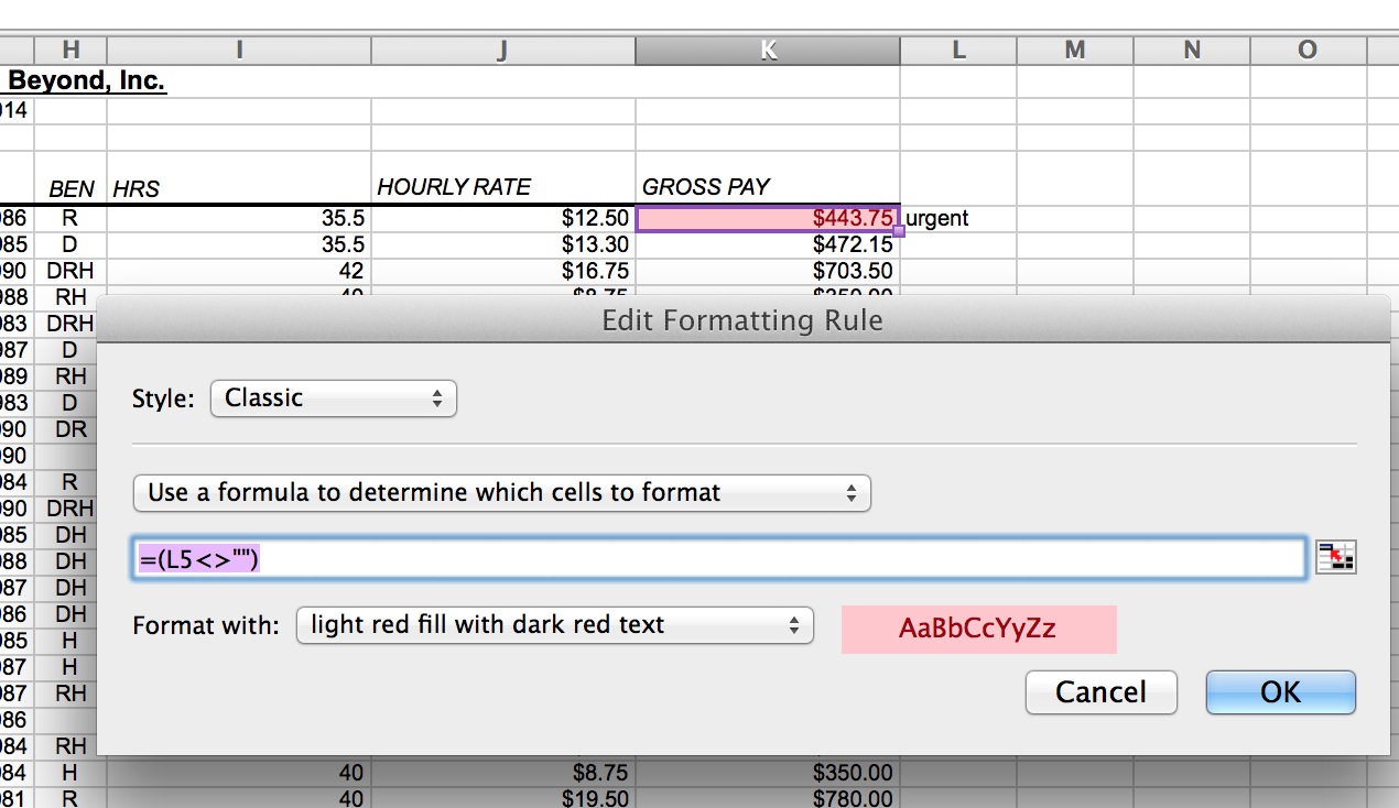
- Choose New Rule.
- Select Use a formula to determine which cells to format.
- Enter your formula. For example,
=A1="Yes". - Click Format and choose your formatting options.
- Press OK to apply the rule.
Your selected cells will now change based on another cell’s value.
Practical Applications
Conditional formatting based on another cell has many practical uses:
- Highlighting overdue tasks: Format tasks based on due dates.
- Tracking project status: Use colors to show progress.
- Inventory management: Flag items needing restocking.
These applications make your data more actionable and easier to understand.
Advanced Techniques
Excel’s Conditional Formatting offers many advanced techniques. These techniques help highlight data based on other cells. This section covers two key areas.
Using Multiple Conditions
Excel lets users apply multiple conditions to format cells. This feature is powerful for complex data analysis. Follow these steps:
- Select the range of cells you want to format.
- Go to the Home tab.
- Click on Conditional Formatting.
- Choose New Rule.
- Select Use a formula to determine which cells to format.
- Enter your first condition formula, for example:
=A1>10. - Click Format to set the formatting style.
- Repeat the process for additional conditions.
Here’s a table summarizing common conditions:
| Condition | Formula | Example |
|---|---|---|
| Greater than | =A1>10 | Values greater than 10 |
| Less than | =A1<5 | Values less than 5 |
| Equal to | =A1=7 | Values equal to 7 |
Combining With Other Excel Features
Combining Conditional Formatting with other Excel features enhances functionality. For example, use it with Data Validation to ensure data integrity.
- Data Validation: Highlight invalid entries.
- VLOOKUP: Format cells based on lookup values.
- PIVOT Tables: Apply formatting to summarized data.
Here’s how to use Conditional Formatting with Data Validation:
- Select the cell range.
- Go to Data tab.
- Click on Data Validation.
- Set your validation criteria, e.g.,
Whole numberbetween1and100. - Apply Conditional Formatting to highlight invalid entries.
These advanced techniques help you get the most out of Excel. Use them to make your data clear and actionable.
Common Issues
Excel Conditional Formatting based on another cell can sometimes be tricky. Users often face common issues that can hinder their workflow. These problems include incorrect formulas, misapplied rules, and unexpected formatting results. Understanding these common issues can help you troubleshoot effectively and avoid potential pitfalls.
Troubleshooting Tips
Follow these tips to solve common issues:
- Check your formulas: Ensure your formulas are correct and referencing the right cells.
- Format consistency: Make sure the formats are consistent across your worksheet.
- Rule order: Conditional formatting rules apply in order. Check the sequence of your rules.
Use these tips to solve issues quickly and efficiently.
Avoiding Common Pitfalls
To avoid common pitfalls, keep these points in mind:
- Use absolute references: Use absolute cell references to avoid issues with cell shifts.
- Clear old rules: Remove outdated rules to prevent conflicts.
- Test your rules: Always test your conditional formatting rules on a sample dataset first.
By following these steps, you can minimize errors and ensure smooth functionality.
| Issue | Solution |
|---|---|
| Incorrect Formula | Double-check your formula syntax and cell references. |
| Misapplied Rules | Ensure that the rules are applied to the correct range of cells. |
| Unexpected Formatting | Review the rule order and test formatting on sample data. |
These solutions address the most common issues users face.
Case Studies
Excel’s Conditional Formatting Based on Another Cell is a powerful tool. It helps visualize data in meaningful ways. Let’s explore some real-world case studies.
Real-world Examples
Consider a sales team tracking their monthly targets. They use Conditional Formatting to highlight achievements:
| Salesperson | Monthly Target | Actual Sales | Status |
|---|---|---|---|
| Jane | $10,000 | $12,000 | Met |
| John | $8,000 | $7,500 | Not Met |
Another example is an attendance sheet. Teachers use Conditional Formatting to mark late students:
- On-time: Green
- Late: Red
Industry-specific Uses
In healthcare, professionals use Conditional Formatting to monitor patient vitals:
- Normal range: Green
- Critical range: Red
Finance teams use it for budget tracking. They highlight overspending areas:
- Under budget: Green
- Over budget: Red
In the retail industry, managers track inventory levels. They use different colors for stock status:
- In stock: Blue
- Low stock: Yellow
- Out of stock: Red
These case studies show how Conditional Formatting makes data actionable. Different industries benefit from this simple yet powerful feature.
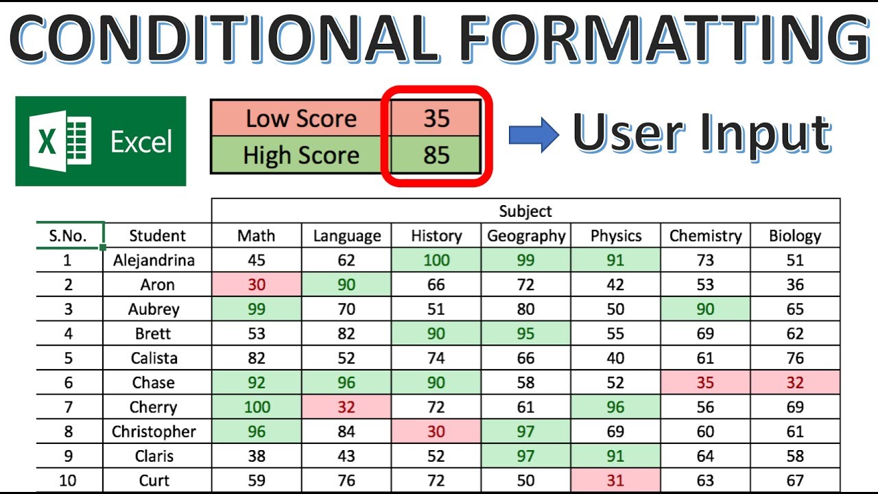
Credit: www.youtube.com
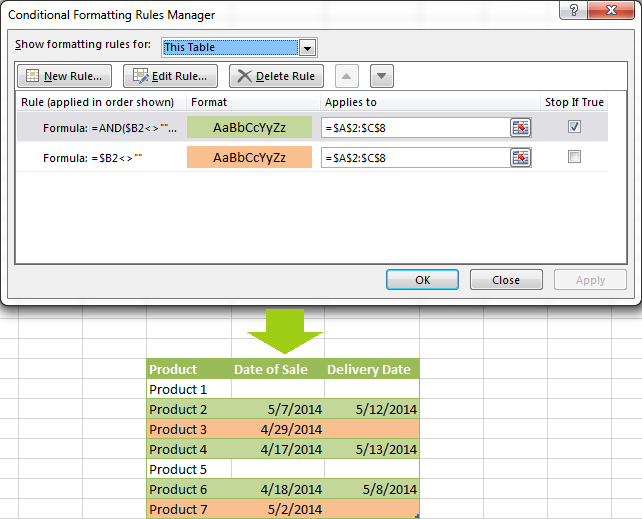
Credit: www.ablebits.com
Frequently Asked Questions
How Do You Use Conditional Formatting In Excel?
To use conditional formatting in Excel, select the cells, go to the “Home” tab, click “Conditional Formatting,” and set your rules.
Can You Base Conditional Formatting On Another Cell?
Yes, you can base conditional formatting on another cell. Use a formula that references the other cell in the rule.
What Is A Formula For Conditional Formatting?
A common formula is =A1=”Text”. This highlights cells based on specific text in another cell.
How Do You Highlight A Row Based On A Cell Value?
To highlight a row, use a formula like =$A1=”Text”. Apply this rule to the entire row range.
Conclusion
Mastering Excel conditional formatting based on another cell can boost your productivity. It’s a powerful tool for data analysis. Applying these techniques makes your spreadsheets more dynamic and insightful. Start experimenting with conditional formatting today. Unlock the full potential of your Excel skills and transform your data presentation.