
To shade every other row in Excel, use the conditional formatting feature. Select your range and apply a formula to format alternating rows.
Excel is a powerful tool for data management and analysis. One useful feature is the ability to shade every other row, which improves readability. This technique is particularly helpful for large datasets. It helps users quickly distinguish between different rows.
The process involves using Excel’s conditional formatting feature. By applying a simple formula, you can easily achieve this effect. Shading every other row not only makes your spreadsheet look professional but also enhances data organization. This guide will help you understand the steps needed to implement this feature. Follow the instructions to make your data visually appealing and easier to read.
Credit: www.simonsezit.com
Preparing Your Excel Sheet
Shading every other row in Excel can make your data easier to read. Preparing your Excel sheet is the first step. Follow these simple steps to make your Excel sheet ready for shading.
Opening Excel
First, open your Excel application. Click on the Excel icon on your desktop or start menu.
If you don’t have an existing file, create a new one. Click on File and then select New. Choose Blank Workbook to start fresh.
Selecting The Data Range
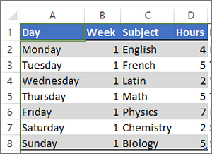
Next, select the data range you want to shade. Click and drag your mouse over the cells.
Ensure you highlight the entire range, including headers if necessary. This helps in applying the shading uniformly.
For large datasets, use the keyboard shortcut Ctrl + Shift + Down Arrow to select quickly. This selects all rows in a column.
| Action | Steps |
|---|---|
| Open Excel | Click on the Excel icon |
| Create New File | File > New > Blank Workbook |
| Select Data Range | Click and drag over the cells |
Now your Excel sheet is ready for shading every other row. These steps ensure your data is correctly prepared for the next phase.
Credit: support.microsoft.com
Using Conditional Formatting
Shading every other row in Excel helps make data more readable. One efficient way to achieve this is by using Conditional Formatting. This method allows you to apply a specific format to cells that meet certain conditions. Follow these simple steps to shade alternate rows using Conditional Formatting.
Accessing Conditional Formatting
First, open your Excel workbook and select the worksheet you want to format. Highlight the range of cells where you want to apply the shading.
Next, go to the Home tab on the Excel ribbon. In the Styles group, click on the Conditional Formatting drop-down menu.
From the drop-down menu, select New Rule. This will open the New Formatting Rule dialog box.
Creating A New Rule
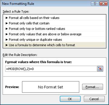
In the New Formatting Rule dialog box, choose Use a formula to determine which cells to format.
In the Format values where this formula is true box, enter the following formula:
=MOD(ROW(),2)=0This formula checks if a row number is even.
Click the Format button to specify the formatting you want to apply. You can choose a fill color to shade the rows.
Once you’ve chosen your formatting options, click OK. Then click OK again in the New Formatting Rule dialog box.
Your worksheet should now show alternate rows shaded in the color you selected.
Customizing Formatting Rules
Want to make your Excel sheet easier to read? One way is by shading every other row. This makes data pop out, making it simpler to scan and analyze. You can use Excel’s conditional formatting feature to achieve this. Let’s explore how to customize these formatting rules.
Formula For Alternating Rows
First, you need a formula to identify alternating rows. Go to your Excel sheet and follow these steps:
- Select the range of cells where you want to apply shading.
- Go to the Home tab, then click on Conditional Formatting.
- Choose New Rule from the dropdown menu.
- In the New Formatting Rule window, select Use a formula to determine which cells to format.
- Enter the formula
=MOD(ROW(),2)=0in the formula box.
This formula tells Excel to shade every other row. The MOD function checks if the row number is even. If it is, the row gets shaded.
Choosing Colors
After setting the formula, you need to choose your colors. Here’s how:
- In the same New Formatting Rule window, click the Format button.
- Go to the Fill tab to select your shading color.
- Choose a color that contrasts well with your text.
- Click OK to apply the color.
You can use different colors to highlight rows. This helps in differentiating data rows and makes your Excel sheet visually appealing.
Here is a simple table to illustrate:
| Row Number | Data | Shading |
|---|---|---|
| 1 | Apple | None |
| 2 | Banana | Shaded |
| 3 | Cherry | None |
| 4 | Date | Shaded |
In this table, every other row is shaded, making it easier to read.
Applying The Rule
Shading every other row in Excel can make your data easier to read. This technique helps to differentiate between rows, making your spreadsheet look professional. Here’s how you can apply the rule efficiently.
Selecting The Range
First, select the range of cells you want to format. Click and drag over the cells to highlight them. You can also use keyboard shortcuts for quicker selection.
Once your cells are highlighted, you are ready to apply the formatting rule. This selection is crucial for the next steps.
Go to the Home tab in the Excel ribbon. Click on Conditional Formatting in the Styles group. A dropdown menu will appear.
Select New Rule from the dropdown menu. In the New Formatting Rule dialog box, choose Use a formula to determine which cells to format.
In the Format values where this formula is true box, enter the following formula:
=MOD(ROW(),2)=0
This formula checks if the row number is even. If true, it applies the format.
Click Format to set the formatting options. Choose your desired fill color and click OK.
Confirming The Rule
After setting the format, click OK in the New Formatting Rule dialog box. Your selected range should now show the shading on every other row.
You can review your rule by going back to Conditional Formatting. Click on Manage Rules to see all applied rules.
Make sure everything looks correct. If needed, you can edit the rule by selecting it and clicking Edit Rule.
Shading every other row is now successfully applied. Your data is more readable and visually appealing.
Editing And Removing Rules
Editing and removing rules in Excel are essential skills. They help you customize and manage your worksheets effectively. Whether you need to modify existing rules or remove conditional formatting, knowing how to do it can save time and enhance your Excel experience.
Modifying Existing Rules
To modify existing rules in Excel, follow these steps:
- Open your Excel workbook.
- Click on the Home tab.
- Go to the Styles group.
- Click on Conditional Formatting.
- Select Manage Rules.
You will see a list of all your rules. Select the rule you want to edit. Click on Edit Rule. Make the necessary changes. Click OK to save.
Removing Conditional Formatting
Removing conditional formatting is straightforward. Here are the steps:
- Open your Excel workbook.
- Navigate to the Home tab.
- Go to the Styles group.
- Click on Conditional Formatting.
- Select Clear Rules.
- Choose from Clear Rules from Selected Cells or Clear Rules from Entire Sheet.
This action removes all formatting rules from the selected cells or the entire sheet.
To remove specific rules, go to Manage Rules. Select the rule you wish to delete. Click on the Delete Rule button. Click OK to finalize.
Tips And Tricks
Shading every other row in Excel can make data easier to read. It helps to highlight important information. Here are some tips and tricks to achieve this easily.
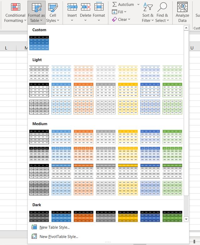
Using Predefined Templates
Excel provides predefined table styles. These styles make it simple to shade alternate rows.
- Select the range of cells you want to format.
- Go to the Home tab.
- Click on Format as Table in the Styles group.
- Choose a style that shades every other row.
Excel will automatically format your table. The shading will alternate as you add more rows.
Advanced Formatting Options
For more control, you can use Conditional Formatting. This method allows custom shading patterns.
- Select the range of cells.
- Navigate to the Home tab.
- Click on Conditional Formatting in the Styles group.
- Choose New Rule.
- Select Use a formula to determine which cells to format.
Click on Format and choose a fill color.
Click OK to apply the rule. The rows will now alternate in color based on your custom settings.
These tips and tricks can help you manage data more effectively in Excel. Use predefined templates for quick results. For more customization, go for advanced formatting options.
Troubleshooting
Shading every other row in Excel is often straightforward. But sometimes, issues arise. These problems can be frustrating. This section will help you troubleshoot common issues and fix mistakes.
Common Issues
Some common issues include:
- Shading does not apply to all rows.
- Rows are shaded incorrectly.
- Formatting disappears after sorting data.
Shading not applying to all rows often happens due to incorrect range selection. Make sure you select the entire range.
Rows shaded incorrectly can occur if your formula is wrong. Double-check the formula used for shading.
Formatting disappears after sorting data is a common problem. This can happen if conditional formatting rules are not set properly.
Fixing Mistakes
Let’s look at how to fix these mistakes.
1. Incorrect Range Selection
To fix this, make sure you:
- Select the entire range you want to shade.
- Check the range in the conditional formatting rules.
2. Incorrect Formula
If rows are shaded incorrectly:
- Double-check your formula.
- Use a correct formula like
=MOD(ROW(),2)=0.
3. Formatting Disappears After Sorting
To prevent this:
- Use “Use a formula to determine which cells to format”.
- Ensure the formula is applied to the entire table.
These steps will help you fix common issues. Follow them to ensure every other row is shaded correctly in Excel.
Credit: support.microsoft.com
Frequently Asked Questions
How Do I Shade Every Other Row In Excel?
To shade every other row in Excel, use Conditional Formatting. Select the range, go to Home > Conditional Formatting > New Rule. Choose “Use a formula to determine which cells to format” and enter the formula =MOD(ROW(),2)=0. Choose your desired formatting and apply.
Can I Alternate Row Colors In Excel?
Yes, you can alternate row colors in Excel using Conditional Formatting. Select your range, then go to Home > Conditional Formatting > New Rule. Use the formula =MOD(ROW(),2)=0 and choose your color. Apply to see alternating row colors.
Why Use Alternating Row Colors In Excel?
Alternating row colors improve readability and make data easier to follow. It helps in distinguishing between rows quickly, especially in large datasets. This technique is particularly useful for presentations and printed reports.
How Do I Remove Shading From Rows In Excel?
To remove shading, select the shaded cells or range, then go to Home > Conditional Formatting > Clear Rules > Clear Rules from Selected Cells. This action will remove any conditional formatting, including shading, from the selected cells.
Conclusion
Mastering how to shade every other row in Excel enhances your data’s readability. This simple technique saves time and effort. Follow these steps to create a visually appealing spreadsheet. Implement these tips, and your Excel skills will surely impress. Keep practicing to become proficient.